A/B Testing Demystified...Part 1: The Science of Fair Comparisons

TL;DR

• ✅ Randomization makes comparisons fair.
• ✅ Hypotheses set the trial: H₀ (no effect) vs H₁ (effect exists).
• ✅ Two errors matter: Type I (false win), Type II (missed win).
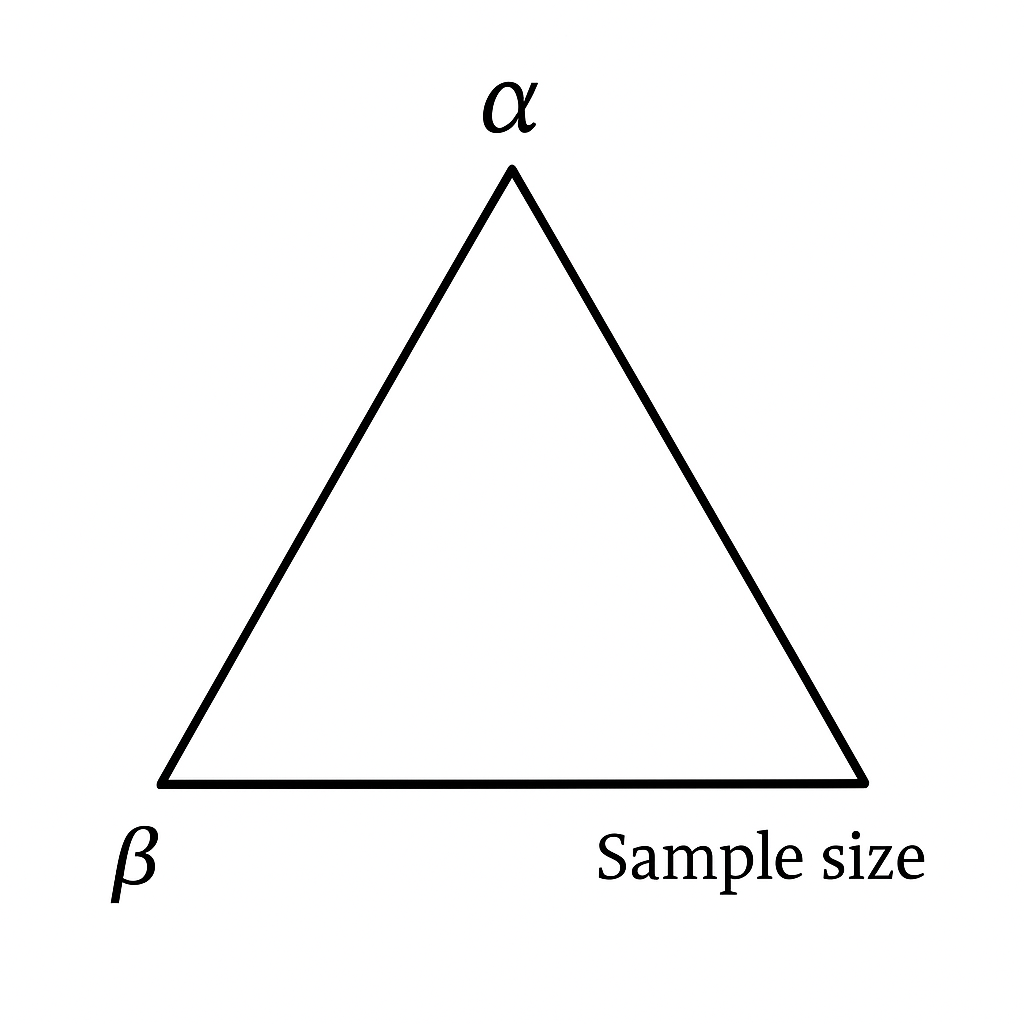
• ✅ Significance (α), Power (1−β), and Sample Size form a triangle — you can’t minimize all at once.
• ✅ Most A/B tests fail because of underpowered sample sizes.

---

1. The Button That Could Change Everything

Should the “Buy Now” button be green or blue?

On the surface, it sounds trivial. Designers will insist one looks modern.
Marketers will swear another converts better. But for a company like Amazon, Netflix, or Booking.com, even a 1% improvement in click-through rate (CTR) can translate to millions of dollars in revenue.

This is the story of A/B testing: a deceptively simple experiment design that underpins how the digital world decides what works.

Yet beneath its simplicity lies a web of statistics, probability, and pitfalls.
Run carelessly, and an A/B test can lie to you convincingly. Run properly, and it becomes your most trusted compass for decision-making.

This series is about doing it properly.

• Part 1 (this article): The scientific backbone — hypotheses, errors, and sample size.
• Part 2: Running tests in practice — messy data, statistical vs business significance, Python demos.
• Part 3: Beyond A/B — Bayesian testing, multi-armed bandits, and scaling experiments in industry.

So let’s start with the foundations.

---

2. Why Not Just Change It and See?

Suppose you roll out the blue button and notice clicks increased the next week.
Does that mean it worked?

Maybe. But maybe not.

• Perhaps it was a holiday weekend and traffic surged.
• Maybe you ran a big ad campaign at the same time.
• Or maybe the users who came in that week were just different.

This is the confounding problem: when outside factors cloud the effect of your change.

Randomization solves it. By flipping a coin and assigning users randomly to green or blue, you ensure that everything else — time of day, device type, region, mood — is balanced across groups.

Any difference you see can now credibly be attributed to the button color.

That’s the essence of A/B testing. But to truly understand it, we need to put it on trial.

---

3. Hypotheses: Putting Ideas on Trial

An A/B test is like a courtroom drama.

• The null hypothesis (H₀) is innocent until proven guilty.
  • There’s no difference between green and blue.
• The alternative hypothesis (H₁) is the prosecution’s claim.
  • The blue button changes user behavior.

We don’t ever “prove” H₀ true. Instead, we ask:
Do we have enough evidence to reject it?

Interpretation:
H₀ is the status quo. H₁ is the possibility of improvement.
A/B testing is a jury trial for your product decisions.

---

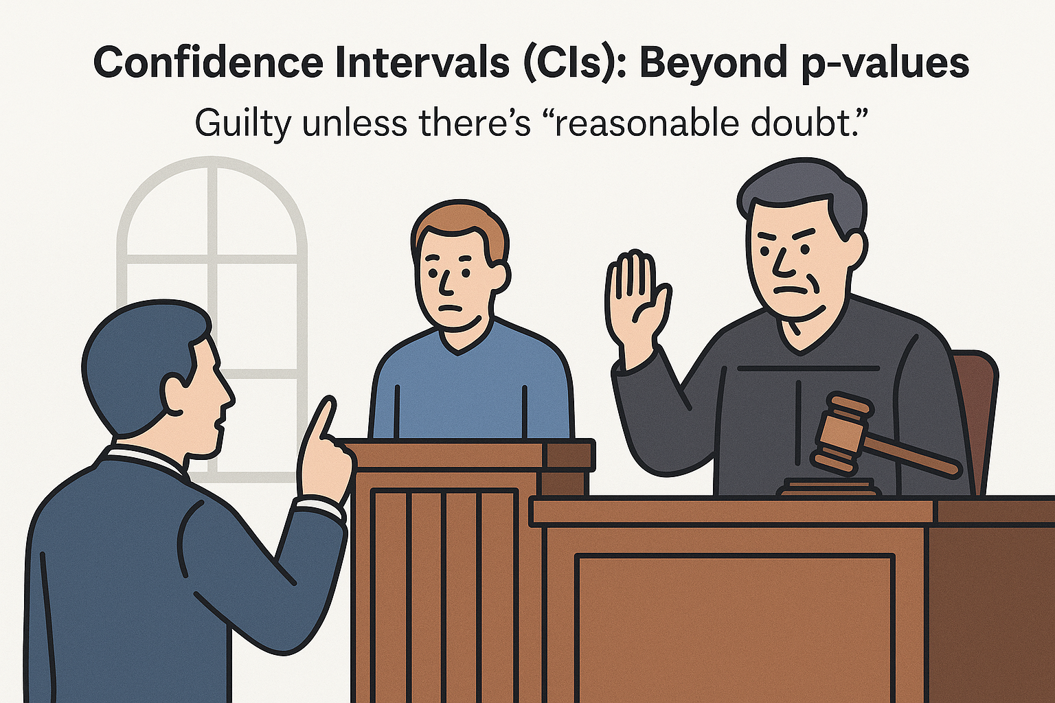
4. Errors: When the Jury Gets It Wrong

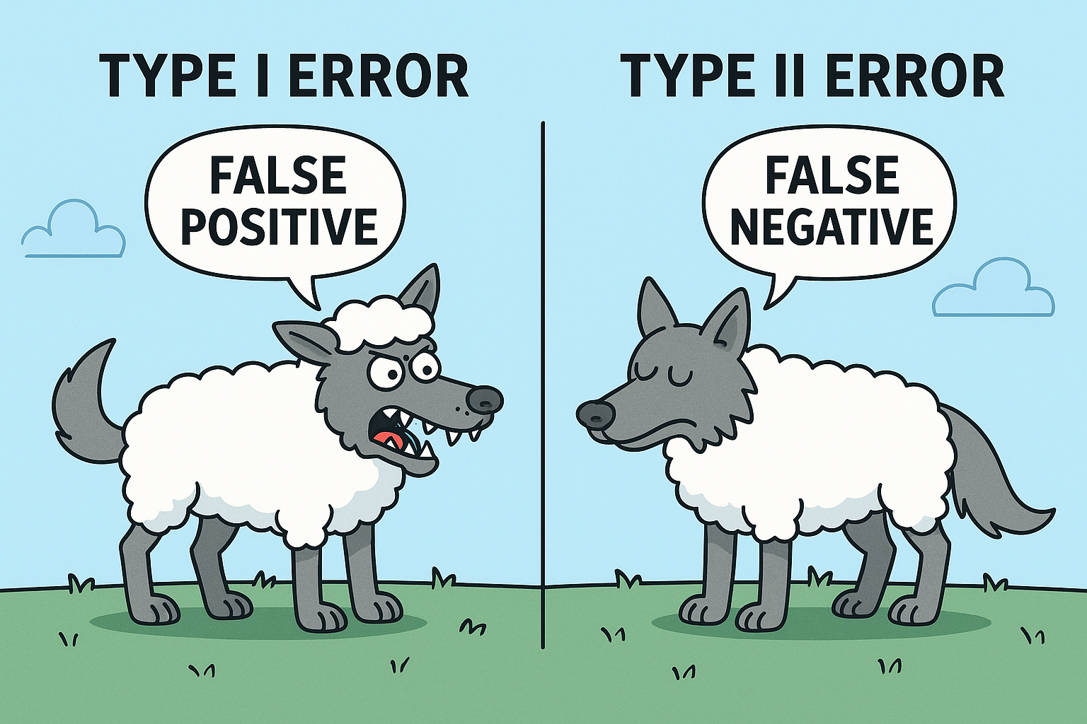
Just like juries, tests can make mistakes. Two kinds, in fact:

Type I Error (α): False Positive

You convict an innocent person.
In A/B: you conclude blue is better when it’s not.

• Typically we set α = 0.05 → a 5% chance of crying wolf.
• This is called the significance level.

Type II Error (β): False Negative

You let the guilty go free.
In A/B: you fail to see that blue really was better.

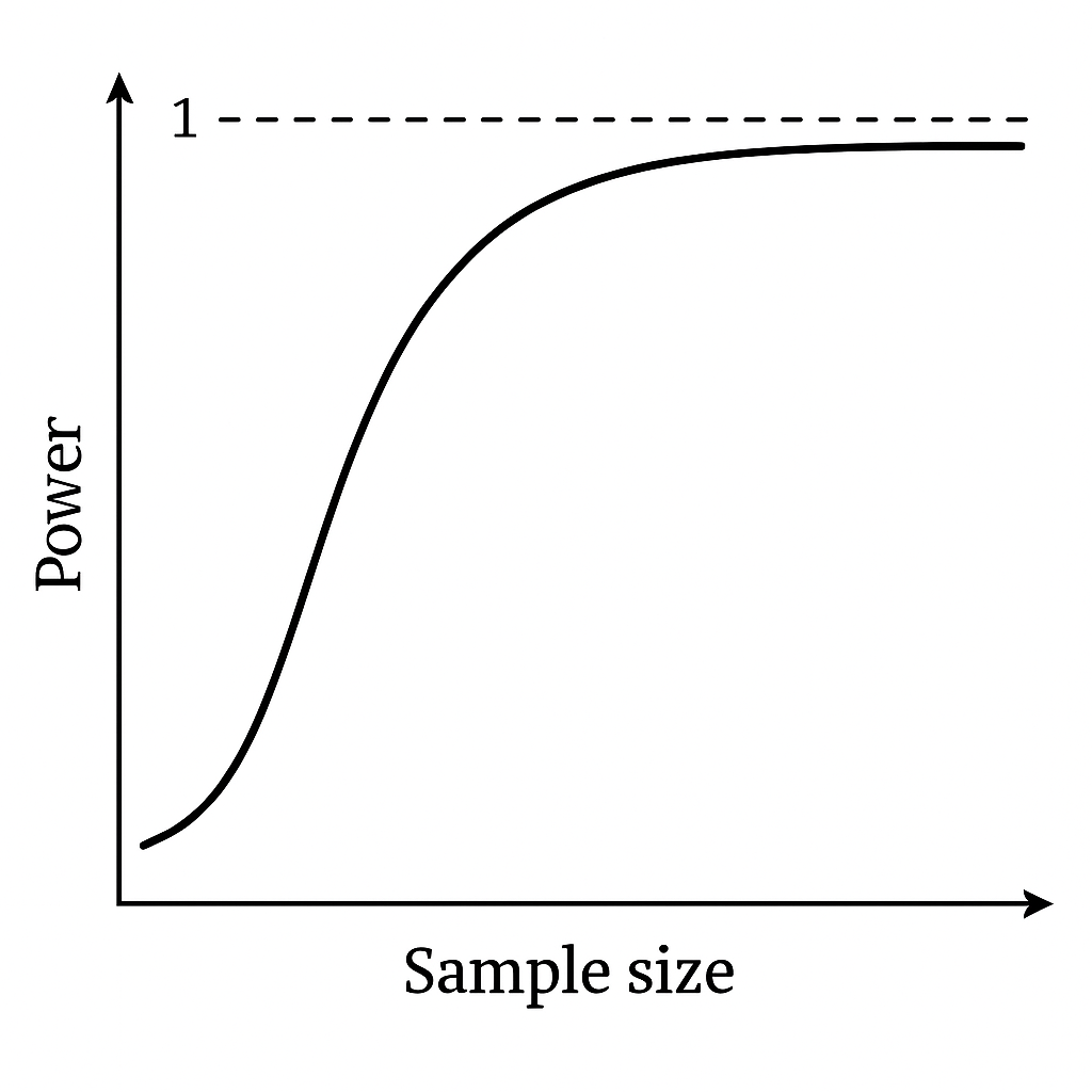
• The probability of avoiding this error is Power = 1 − β.
• Power tells us: if there is a real effect, how likely are we to catch it?
• Industry standard: Power = 0.8 (80%).

---

5. Trade-offs Between α, β, and Sample Size

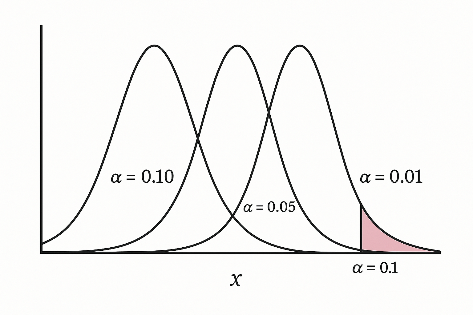
Changing α is like changing the rules of the courtroom:

• α = 0.10 (lenient): You’ll catch more true improvements, but also more false alarms.
• α = 0.05 (standard): Balanced — some risk of error, but manageable.
• α = 0.01 (strict): Very cautious — fewer false wins, but you’ll miss many small true lifts.

Power is your flashlight in a dark room — brighter power shows more truth, but it costs more data.

• 50% Power: like flipping a coin — useless.
• 80% Power (standard): You’ll detect most real effects.
• 90% Power: Better, but requires much larger samples.

This is the impossible triangle of experiment design:

---

6. Sample Size: Why Small Tests Lie

Here’s the dirty secret: most A/B tests are underpowered.

Someone runs an experiment with 500 users, sees blue “win,” and celebrates. But statistics doesn’t work that way.

We need enough data to reduce noise.

Worked Example

• Baseline CTR = 10%.
• Expected CTR after change = 11%.
• Significance α = 0.05.
• Power = 0.8.

Formula (two-sample proportions test):

$$ n = \frac{2 \cdot (Z_{1-\alpha/2} + Z_{1-\beta})^2 \cdot p(1-p)}{\Delta^2} $$

Where:

• $p = \frac{p_1 + p_2}{2} = 0.105$
• $\Delta = p_2 - p_1 = 0.01$
• $Z_{1-\alpha/2} = 1.96$ (for α = 0.05)
• $Z_{1-\beta} = 0.84$ (for power = 0.8)

Plugging in:

$$ n = \frac{2 \cdot (1.96 + 0.84)^2 \cdot 0.105 \cdot 0.895}{0.01^2} $$

$$ n \approx 15,724 \text{ users per group} $$

So to detect a 1% lift, you’d need ~31,500 users total.

Python Check

from statsmodels.stats.power import NormalIndPower
import math

alpha = 0.05
power = 0.8
p1, p2 = 0.10, 0.11

def cohen_h(p1, p2):
    return 2 * (math.asin(math.sqrt(p1)) - math.asin(math.sqrt(p2)))

h = cohen_h(p1, p2)
analysis = NormalIndPower()
n = analysis.solve_power(effect_size=h, alpha=alpha, power=power, ratio=1)

print(f"Required sample size per group: {math.ceil(n)}")

7. Confidence Intervals (CIs): Beyond p-values

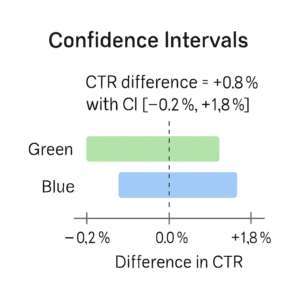
A 95% confidence interval doesn’t mean “there’s a 95% chance the true effect is inside this range.”

It means: if we repeated the experiment many times, 95% of the calculated intervals would contain the true effect.

• Example: CTR difference = +0.8% with CI [−0.2%, +1.8%].
• Interpretation: The true effect might be negative — so we can’t claim a win.

---

8. Sidebar: A Bit of History

In 1935, statistician Ronald Fisher described the “Lady Tasting Tea” experiment.
A woman claimed she could tell whether milk or tea was poured first. Fisher designed a controlled experiment to test her.

This simple test introduced the very concepts of null hypothesis and statistical evidence we use today.

---

9. Simpson’s Paradox (Teaser for Part 2)

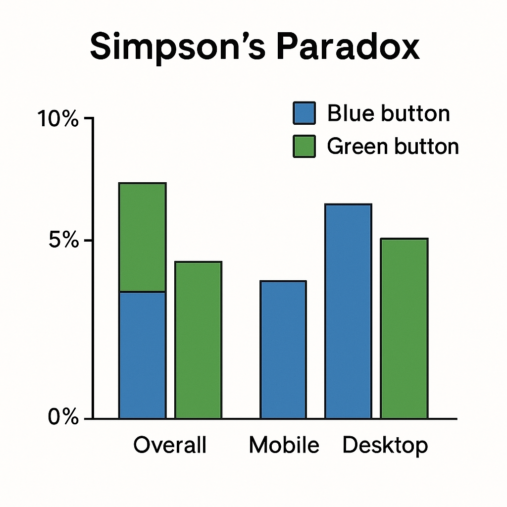
Sometimes, aggregated results can mislead.

• Overall, blue button looks worse.
• But when you break it down by device (mobile vs desktop), blue wins in both.

This reversal is Simpson’s Paradox, and we’ll see why it matters in Part 2 when we dive into messy, real-world experiments.

---

10. Common Pitfalls in Foundations

1. Peeking Too Early

   • Checking results halfway inflates false positives.

2. Small Sample Fallacy

   • Running with a few hundred users → unreliable swings.

3. Multiple Comparisons

   • Testing 10 variants without correction inflates error risk.

---

11. Practical Guidance

Scenario	α	Power	Notes
Medical trial	0.01	0.9	Life/death stakes → minimize false claims
UX design tweak	0.05	0.8	Balanced, industry standard
Exploratory test	0.10	0.8	Okay to be loose if just generating ideas

---

Up for a challenge?

If your baseline CTR were 5% and you wanted to detect a +0.5% lift,
how many users would you need?

(Hint: use the sample size formula - the number is huge.)

What’s the best or worst A/B test you’ve seen in practice?
Share your stories with us and we will feature them in Part 3!